Examples for config.yml file

Configuration file config.yml use YAML (https://yaml.org) format to describe decay process.

The main parts of config.yml is decay and particle.

The decay part describe the particle (or an id of a list of particle) decay into which particles, it can be a list of a list of list. A list means that there is ony one decay mode, A list of list is the list of possible decay mode. The list item can be the particle name (or a dict to describe the decay parameters). All name should appear in particle part.

The particle part describe the parameters of particles. There are two special parts $top and $finals describe the top and finals particles. The other parts are lists of particle name or dicts of particle parameters. The list is the same type particle in decay part. The dict is the parameters of the particle name.

config_str = """

decay:
    A:
       - [R1, B]
       - [R2, C]
       - [R3, D]
    R1: [C, D]
    R2: [B, D]
    R3: [B, C]

particle:
    $top:
       A: { mass: 1.86, J: 0, P: -1}
    $finals:
       B: { mass: 0.494, J: 0, P: -1}
       C: { mass: 0.139, J: 0, P: -1}
       D: { mass: 0.139, J: 0, P: -1}
    R1: [ R1_a, R1_b ]
    R1_a: { mass: 0.7, width: 0.05, J: 1, P: -1}
    R1_b: { mass: 0.5, width: 0.05, J: 0, P: +1}
    R2: { mass: 0.824, width: 0.05, J: 0, P: +1}
    R3: { mass: 0.824, width: 0.05, J: 0, P: +1}

"""

The config file can be loaded by yaml library.

import matplotlib.pyplot as plt
import yaml

from tf_pwa.config_loader import ConfigLoader
from tf_pwa.histogram import Hist1D

config = ConfigLoader(yaml.full_load(config_str))

We set parameters to a blance value. And we can generate some toy data and calclute the weights

input_params = {
    "A->R1_a.BR1_a->C.D_total_0r": 6.0,
    "A->R1_b.BR1_b->C.D_total_0r": 1.0,
    "A->R2.CR2->B.D_total_0r": 2.0,
    "A->R3.DR3->B.C_total_0r": 1.0,
}
config.set_params(input_params)

data = config.generate_toy(1000)
phsp = config.generate_phsp(10000)

# You can also fit the data fit to the data
fit_result = config.fit([data], [phsp])
err = config.get_params_error(fit_result, [data], [phsp])

Out:

6.8%[▓▓▓>----------------------------------------------] 0.32/4.75s eff: 90.000000%
95.3%[▓▓▓▓▓▓▓▓▓▓▓▓▓▓▓▓▓▓▓▓▓▓▓▓▓▓▓▓▓▓▓▓▓▓▓▓▓▓▓▓▓▓▓▓▓▓▓>--] 1.26/1.32s eff: 5.641864%
99.9%[▓▓▓▓▓▓▓▓▓▓▓▓▓▓▓▓▓▓▓▓▓▓▓▓▓▓▓▓▓▓▓▓▓▓▓▓▓▓▓▓▓▓▓▓▓▓▓▓▓>] 1.58/1.58s eff: 4.919047%
99.9%[▓▓▓▓▓▓▓▓▓▓▓▓▓▓▓▓▓▓▓▓▓▓▓▓▓▓▓▓▓▓▓▓▓▓▓▓▓▓▓▓▓▓▓▓▓▓▓▓▓>] 1.85/1.85s eff: 4.891171%
99.9%[▓▓▓▓▓▓▓▓▓▓▓▓▓▓▓▓▓▓▓▓▓▓▓▓▓▓▓▓▓▓▓▓▓▓▓▓▓▓▓▓▓▓▓▓▓▓▓▓▓>] 2.13/2.13s eff: 4.885914%
100.2%[▓▓▓▓▓▓▓▓▓▓▓▓▓▓▓▓▓▓▓▓▓▓▓▓▓▓▓▓▓▓▓▓▓▓▓▓▓▓▓▓▓▓▓▓▓▓▓▓▓▓>] 2.40/2.40s eff: 4.880668%
100.0%[▓▓▓▓▓▓▓▓▓▓▓▓▓▓▓▓▓▓▓▓▓▓▓▓▓▓▓▓▓▓▓▓▓▓▓▓▓▓▓▓▓▓▓▓▓▓▓▓▓▓] 2.40/2.40s  eff: 4.890059%
Using Model_old
decay chains included:
   [A->R1_a+B, R1_a->C+D]  ls:  ((1, 1),) ((1, 0),)
   [A->R1_b+B, R1_b->C+D]  ls:  ((0, 0),) ((0, 0),)
   [A->R2+C, R2->B+D]  ls:  ((0, 0),) ((0, 0),)
   [A->R3+D, R3->B+C]  ls:  ((0, 0),) ((0, 0),)

########### initial parameters
{
  "R1_a_mass": 0.7,
  "R1_a_width": 0.05,
  "R1_b_mass": 0.5,
  "R1_b_width": 0.05,
  "R2_mass": 0.824,
  "R2_width": 0.05,
  "R3_mass": 0.824,
  "R3_width": 0.05,
  "A->R1_a.BR1_a->C.D_total_0r": 6.0,
  "A->R1_a.BR1_a->C.D_total_0i": 0.0,
  "A->R1_a.B_g_ls_0r": 1.0,
  "A->R1_a.B_g_ls_0i": 0.0,
  "R1_a->C.D_g_ls_0r": 1.0,
  "R1_a->C.D_g_ls_0i": 0.0,
  "A->R1_b.BR1_b->C.D_total_0r": 1.0,
  "A->R1_b.BR1_b->C.D_total_0i": -1.277353768539327,
  "A->R1_b.B_g_ls_0r": 1.0,
  "A->R1_b.B_g_ls_0i": 0.0,
  "R1_b->C.D_g_ls_0r": 1.0,
  "R1_b->C.D_g_ls_0i": 0.0,
  "A->R2.CR2->B.D_total_0r": 2.0,
  "A->R2.CR2->B.D_total_0i": -0.485876286050027,
  "A->R2.C_g_ls_0r": 1.0,
  "A->R2.C_g_ls_0i": 0.0,
  "R2->B.D_g_ls_0r": 1.0,
  "R2->B.D_g_ls_0i": 0.0,
  "A->R3.DR3->B.C_total_0r": 1.0,
  "A->R3.DR3->B.C_total_0i": 0.8842336126201742,
  "A->R3.D_g_ls_0r": 1.0,
  "A->R3.D_g_ls_0i": 0.0,
  "R3->B.C_g_ls_0r": 1.0,
  "R3->B.C_g_ls_0i": 0.0
}
initial NLL:  tf.Tensor(-883.5568360919951, shape=(), dtype=float64)
nll_grad  cost time: 0.19311881065368652
nll_grad  cost time: 0.19325923919677734
nll_grad  cost time: 0.19495820999145508
tf.Tensor(-884.7452754760698, shape=(), dtype=float64)
nll_grad  cost time: 0.19398260116577148
nll_grad  cost time: 0.19400429725646973
tf.Tensor(-885.3377760548683, shape=(), dtype=float64)
nll_grad  cost time: 0.1975727081298828
nll_grad  cost time: 0.1950387954711914
tf.Tensor(-885.4720788351624, shape=(), dtype=float64)
nll_grad  cost time: 0.19519495964050293
nll_grad  cost time: 0.19512510299682617
tf.Tensor(-885.5145342921141, shape=(), dtype=float64)
nll_grad  cost time: 0.19577527046203613
nll_grad  cost time: 0.1947486400604248
tf.Tensor(-885.5202098548189, shape=(), dtype=float64)
nll_grad  cost time: 0.19407367706298828
nll_grad  cost time: 0.19347095489501953
tf.Tensor(-885.5652686515696, shape=(), dtype=float64)
nll_grad  cost time: 0.19511103630065918
tf.Tensor(-885.6075834503208, shape=(), dtype=float64)
nll_grad  cost time: 0.1939382553100586
tf.Tensor(-885.6279191839421, shape=(), dtype=float64)
nll_grad  cost time: 0.19423198699951172
tf.Tensor(-885.6279309510765, shape=(), dtype=float64)
Optimization terminated successfully.
         Current function value: -885.627931
         Iterations: 9
         Function evaluations: 16
         Gradient evaluations: 16
      fun: -885.6279309510765
 hess_inv: array([[ 3.62438507e-03, -6.47723574e-04,  5.56687917e-03,
        -1.93792742e-04,  3.45439502e-03, -5.28518298e-04],
       [-6.47723574e-04,  1.54563017e-02,  8.81812271e-05,
         1.58556669e-03, -5.54612459e-04,  5.96316763e-03],
       [ 5.56687917e-03,  8.81812271e-05,  1.44078175e-02,
        -1.05113203e-03,  7.34045599e-03, -5.35103146e-04],
       [-1.93792742e-04,  1.58556669e-03, -1.05113203e-03,
         1.10922681e-02, -9.33802258e-04,  1.73789454e-03],
       [ 3.45439502e-03, -5.54612459e-04,  7.34045599e-03,
        -9.33802258e-04,  7.39812207e-03, -6.04824940e-04],
       [-5.28518298e-04,  5.96316763e-03, -5.35103146e-04,
         1.73789454e-03, -6.04824940e-04,  1.45291313e-02]])
      jac: array([-2.77927883e-04,  1.03858335e-04,  7.23740794e-04, -5.02737748e-05,
        4.13908850e-04, -1.72860937e-06])
  message: 'Optimization terminated successfully.'
     nfev: 16
      nit: 9
     njev: 16
   status: 0
  success: True
        x: array([ 0.94063462, -1.13749413,  1.98873154, -0.47855058,  1.01372769,
        0.85396342])
fit  cost time: 3.3298568725585938
Using Model_old
Time for calculating errors: 0.3742196559906006
hesse_error: [0.060722102736702394, 0.12372817653870379, 0.11942553177097125, 0.10511854671430812, 0.0854569580040078, 0.12042908345896024]

we can see that thre fit results consistant with inputs, the first one is fixed.

for var in input_params:
    print(
        f"in: {input_params[var]} => out: {fit_result.params[var]} +/- {err.get(var, 0.)}"
    )

Out:

in: 6.0 => out: 6.0 +/- 0.0
in: 1.0 => out: 0.9406346153261764 +/- 0.060722102736702394
in: 2.0 => out: 1.988731540372574 +/- 0.11942553177097125
in: 1.0 => out: 1.0137276945522056 +/- 0.0854569580040078

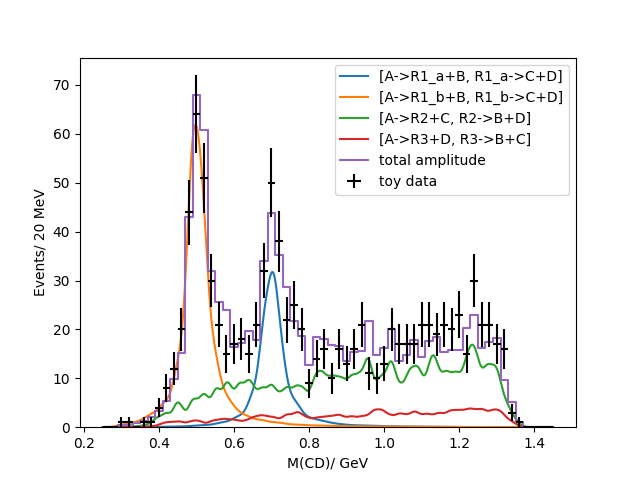
We can use the amplitude to plot the fit results

amp = config.get_amplitude()
weight = amp(phsp)
partial_weight = amp.partial_weight(phsp)

We can plot the data, Hist1D include some plot method base on matplotlib.

data_hist = Hist1D.histogram(
    data.get_mass("(C, D)"), bins=60, range=(0.25, 1.45)
)

mass_phsp = phsp.get_mass("(C, D)")
phsp_hist = Hist1D.histogram(
    mass_phsp, weights=weight, bins=60, range=(0.25, 1.45)
)
scale = phsp_hist.scale_to(data_hist)

pw_hist = []
for w in partial_weight:
    # here we used more bins for a smooth plot
    hist = Hist1D.histogram(
        mass_phsp, weights=w, bins=60 * 2, range=(0.25, 1.45)
    )
    pw_hist.append(scale * hist * 2)

Then we can plot the histogram into matplotlib

for hist, dec in zip(pw_hist, config.get_decay()):
    hist.draw_kde(label=str(dec))
phsp_hist.draw(label="total amplitude")
data_hist.draw_error(label="toy data", color="black")

plt.legend()
plt.ylim((0, None))
plt.xlabel("M(CD)/ GeV")
plt.ylabel("Events/ 20 MeV")
plt.show()