Available Resonances Model
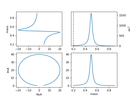
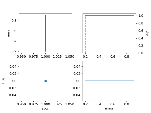
simple particle model for mass, (used in expr)
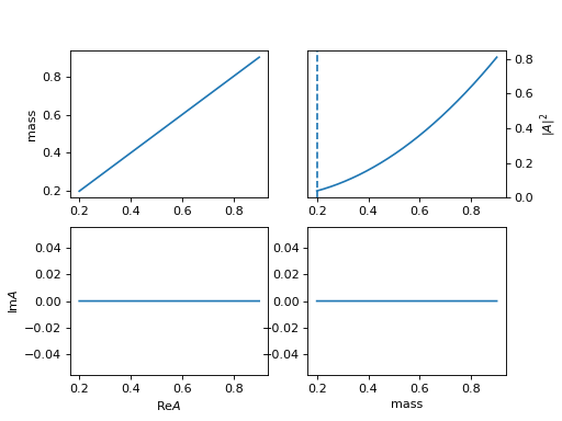
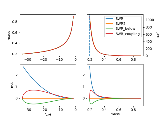
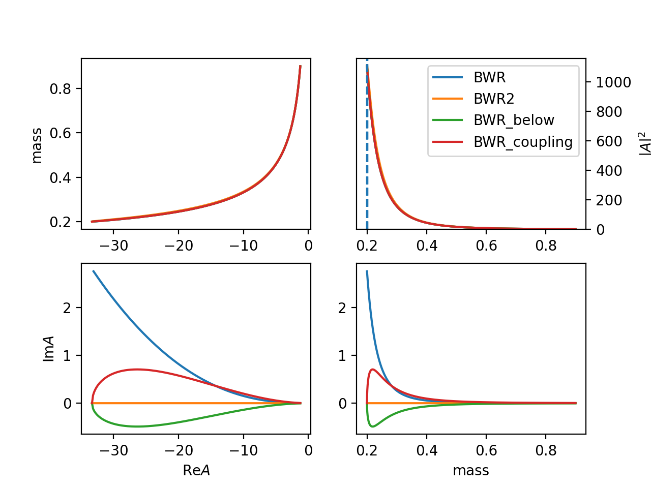
"BWR2"(ParticleBWR2)\[R(m) = \frac{1}{m_0^2 - m^2 - i m_0 \Gamma(m)}\]The difference of
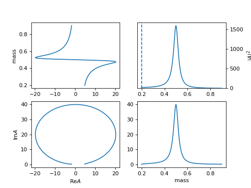
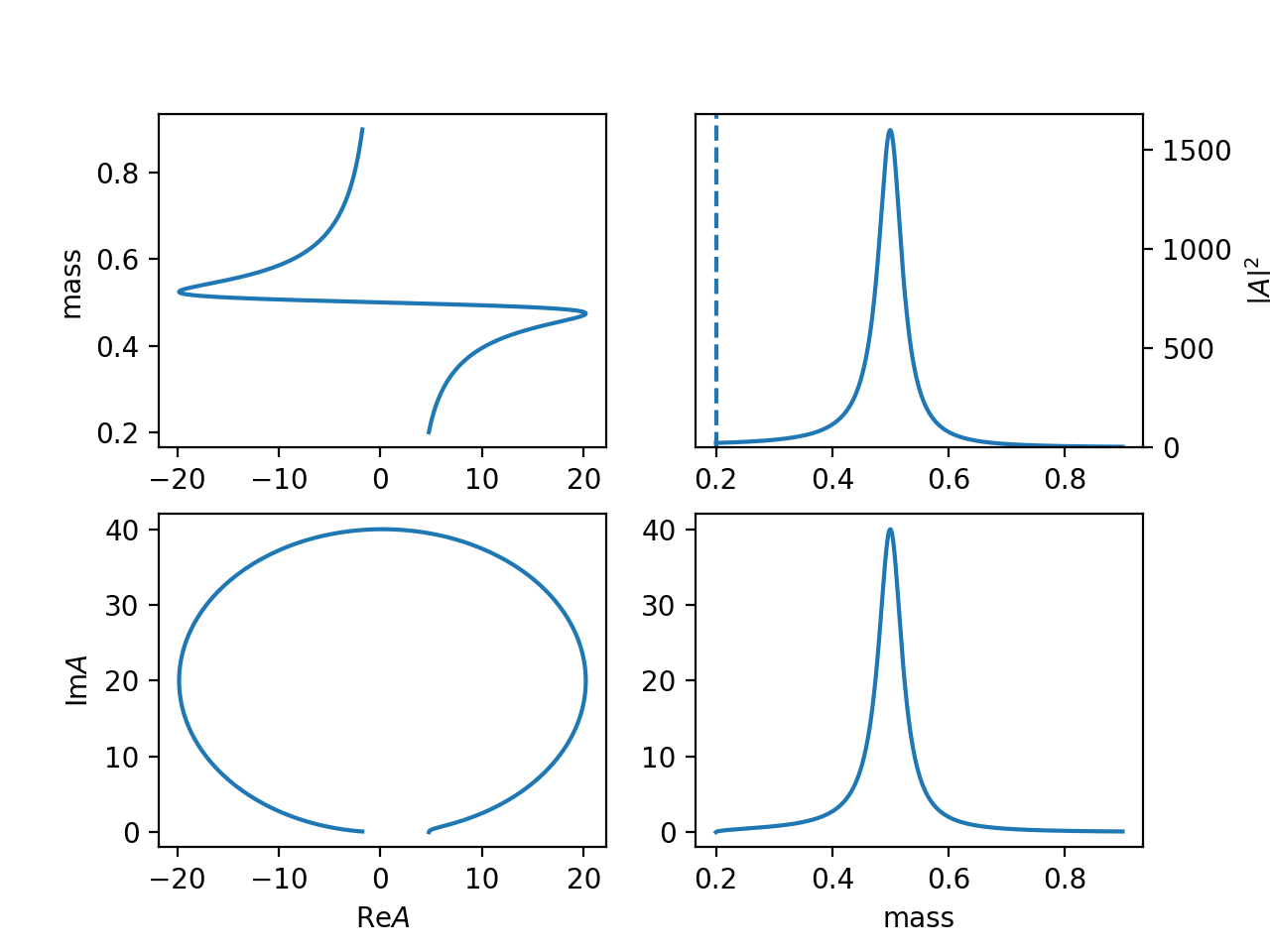
BWR,BWR2is the behavior when mass is below the threshold ( \(m_0 = 0.1 < 0.1 + 0.1 = m_1 + m_2\)).(Source code, png, hires.png, pdf)

"BWR_below"(ParticleBWRBelowThreshold)\[R(m) = \frac{1}{m_0^2 - m^2 - i m_0 \Gamma(m)}\]"BWR_coupling"(ParticleBWRCoupling)Force \(q_0=1/d\) to avoid below theshold condition for
BWRmodel, and remove other constant parts, then the \(\Gamma_0\) is coupling parameters.\[R(m) = \frac{1}{m_0^2 - m^2 - i m_0 \Gamma_0 \frac{q}{m} q^{2l} B_L'^2(q, 1/d, d)}\](Source code, png, hires.png, pdf)
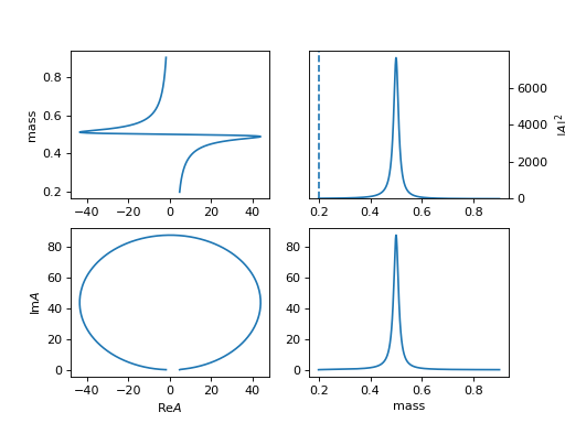
"BWR_normal"(ParticleBWR_normal)\[R(m) = \frac{\sqrt{m_0 \Gamma(m)}}{m_0^2 - m^2 - i m_0 \Gamma(m)}\]"GS_rho"(ParticleGS)Gounaris G.J., Sakurai J.J., Phys. Rev. Lett., 21 (1968), pp. 244-247
c_daug2Mass: mass for daughter particle 2 (\(\pi^{+}\)) 0.13957039c_daug3Mass: mass for daughter particle 3 (\(\pi^{0}\)) 0.1349768\[R(m) = \frac{1 + D \Gamma_0 / m_0}{(m_0^2 -m^2) + f(m) - i m_0 \Gamma(m)}\]\[f(m) = \Gamma_0 \frac{m_0 ^2 }{q_0^3} \left[q^2 [h(m)-h(m_0)] + (m_0^2 - m^2) q_0^2 \frac{d h}{d m}|_{m0} \right]\]\[h(m) = \frac{2}{\pi} \frac{q}{m} \ln \left(\frac{m+q}{2m_{\pi}} \right)\]\[\frac{d h}{d m}|_{m0} = h(m_0) [(8q_0^2)^{-1} - (2m_0^2)^{-1}] + (2\pi m_0^2)^{-1}\]\[D = \frac{f(0)}{\Gamma_0 m_0} = \frac{3}{\pi}\frac{m_\pi^2}{q_0^2} \ln \left(\frac{m_0 + 2q_0}{2 m_\pi }\right) + \frac{m_0}{2\pi q_0} - \frac{m_\pi^2 m_0}{\pi q_0^3}\]"BW"(ParticleBW)"LASS"(ParticleLass)\[R(m) = \frac{m}{q cot \delta_B - i q} + e^{2i \delta_B}\frac{m_0 \Gamma_0 \frac{m_0}{q_0}} {(m_0^2 - m^2) - i m_0\Gamma_0 \frac{q}{m}\frac{m_0}{q_0}}\]\[cot \delta_B = \frac{1}{a q} + \frac{1}{2} r q\]\[e^{2i\delta_B} = \cos 2 \delta_B + i \sin 2\delta_B = \frac{cot^2\delta_B -1 }{cot^2 \delta_B +1} + i \frac{2 cot \delta_B }{cot^2 \delta_B +1 }\]"one"(ParticleOne)"exp"(ParticleExp)\[R(m) = e^{-|a| m}\]"exp_com"(ParticleExp)"KMatrixSingleChannel"(KmatrixSingleChannelParticle)K matrix model for single channel multi pole.
\[K = \sum_{i} \frac{m_i \Gamma_i(m)}{m_i^2 - m^2 }\]\[P = \sum_{i} \frac{\beta_i m_0 \Gamma_0 }{ m_i^2 - m^2}\]the barrier factor is included in gls
\[R(m) = (1-iK)^{-1} P\]"KMatrixSplitLS"(KmatrixSplitLSParticle)K matrix model for single channel multi pole and the same channel with different (l, s) coupling.
\[K_{a,b} = \sum_{i} \frac{m_i \sqrt{\Gamma_{a,i}(m)\Gamma_{b,i}(m)}}{m_i^2 - m^2 }\]\[P_{b} = \sum_{i} \frac{\beta_i m_0 \Gamma_{b,i0} }{ m_i^2 - m^2}\]the barrier factor is included in gls
\[R(m) = (1-iK)^{-1} P\]"BWR_LS"(ParticleBWRLS)Breit Wigner with split ls running width
\[R_i (m) = \frac{g_i}{m_0^2 - m^2 - im_0 \Gamma_0 \frac{\rho}{\rho_0} (\sum_{i} g_i^2)}\], \(\rho = 2q/m\), the partial width factor is
\[g_i = \gamma_i \frac{q^l}{q_0^l} B_{l_i}'(q,q_0,d)\]and keep normalize as
\[\sum_{i} \gamma_i^2 = 1.\]The normalize is done by (\(\cos \theta_0, \sin\theta_0 \cos \theta_1, \cdots, \prod_i \sin\theta_i\))
"interp"(Interp)
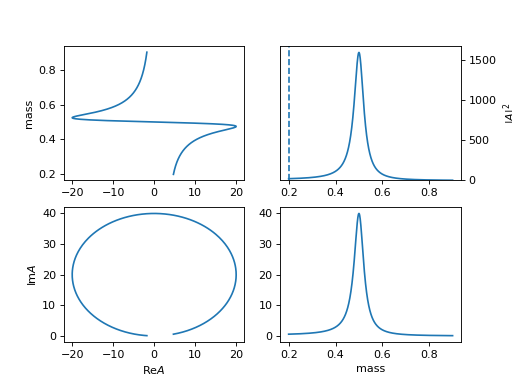

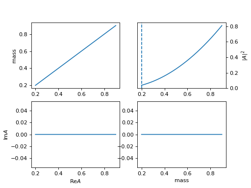
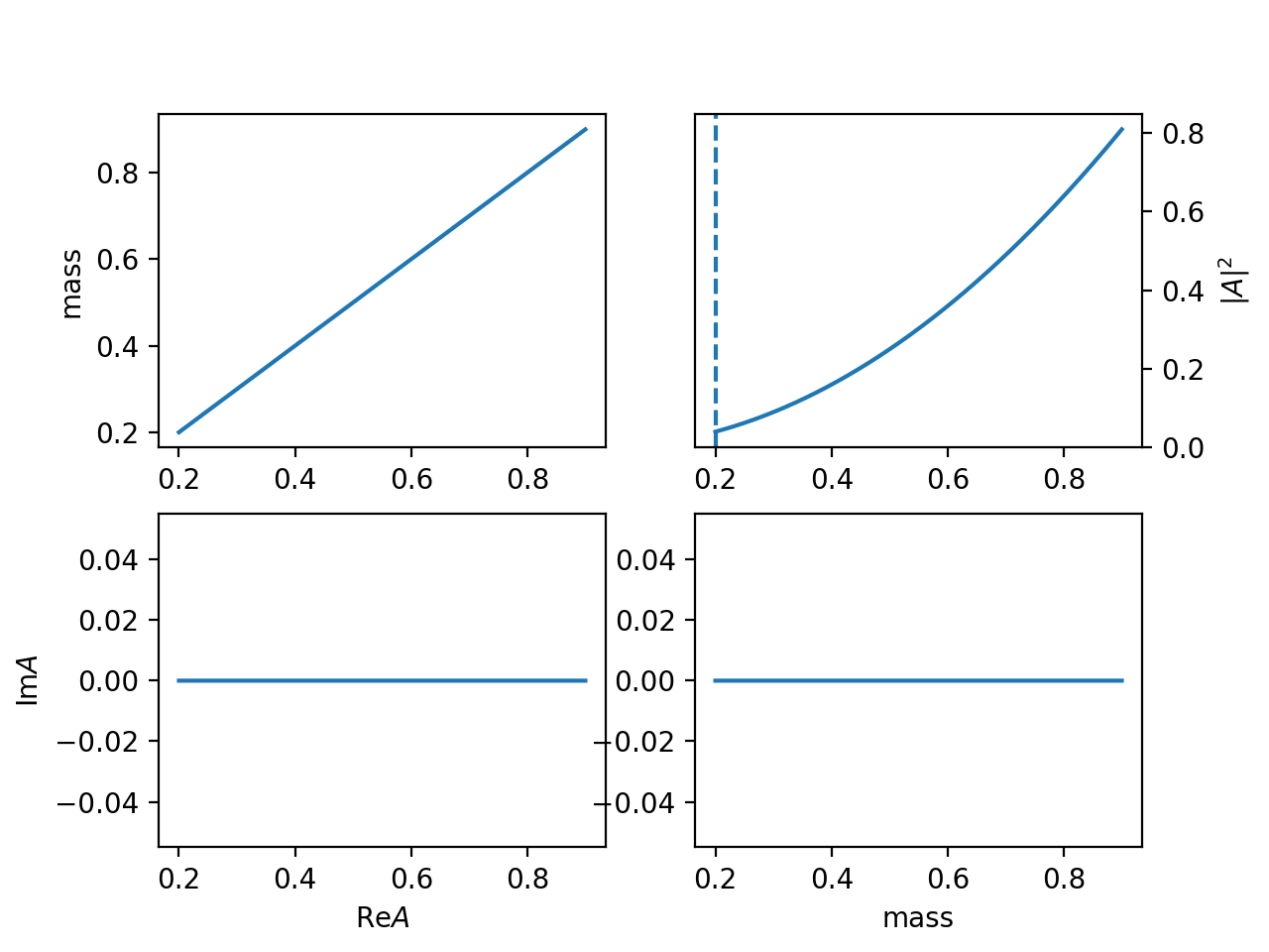

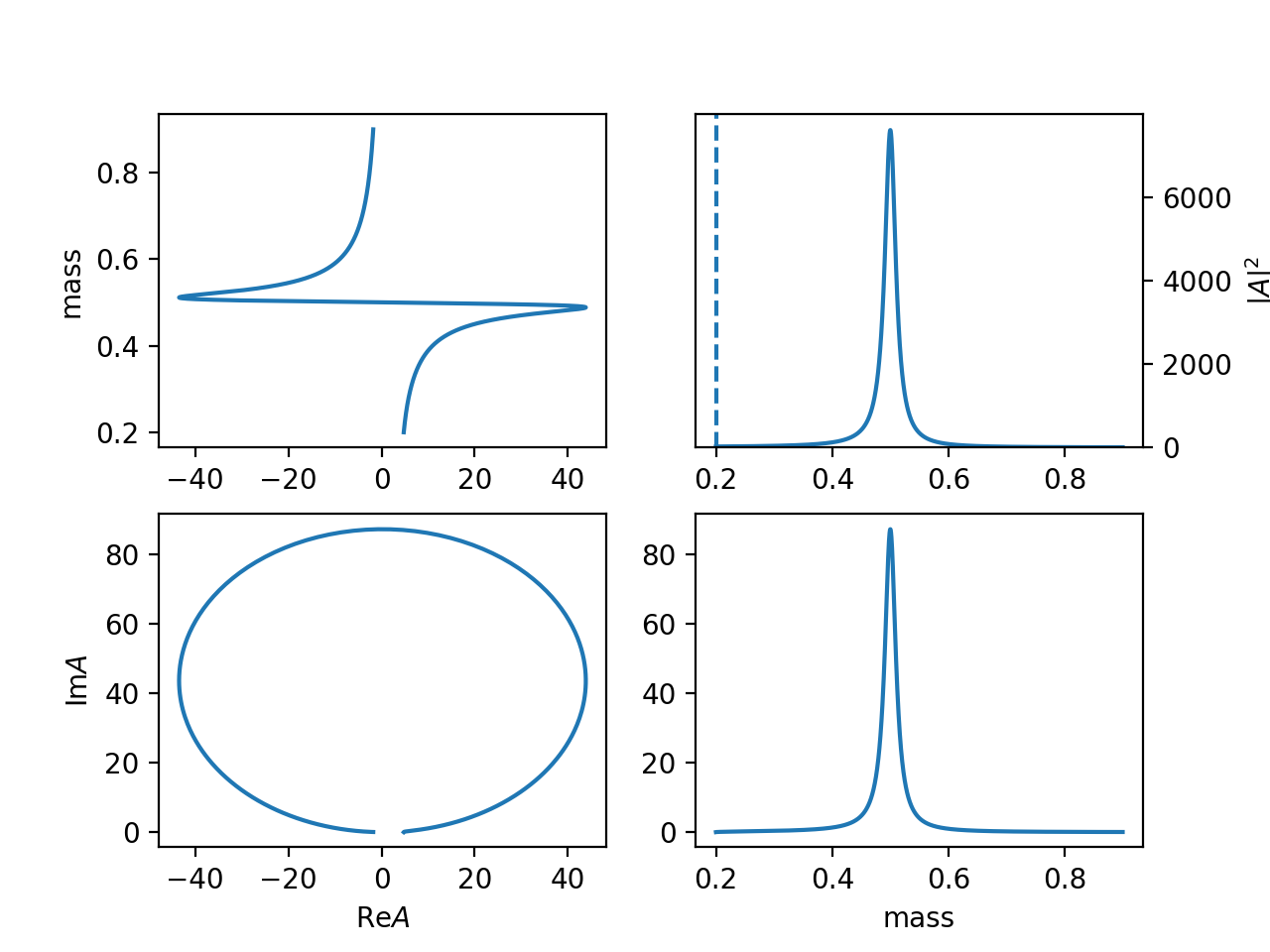


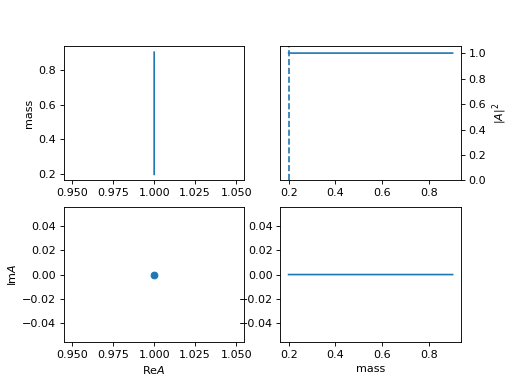
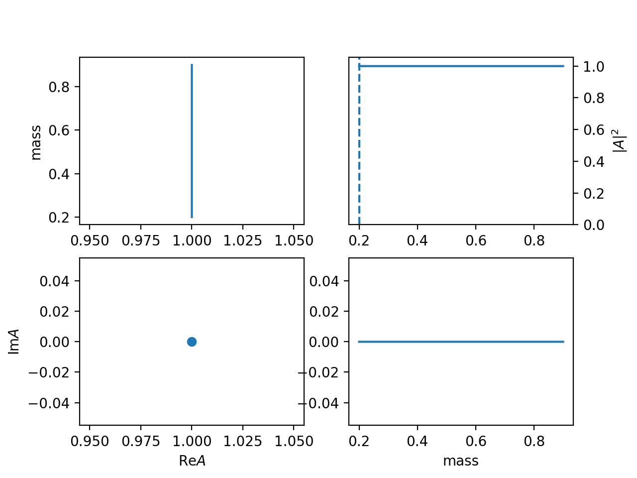


linear interpolation for real number
"interp_c"(Interp)
linear interpolation for complex number
"spline_c"(Interp1DSpline)
Spline interpolation function for model independent resonance
"interp1d3"(Interp1D3)
Piecewise third order interpolation
"interp_lagrange"(Interp1DLang)
Lagrange interpolation
"interp_hist"(InterpHist)
Interpolation for each bins as constant
"hist_idx"(InterpHistIdx)
Interpolation for each bins as constant
"spline_c_idx"(Interp1DSplineIdx)
Spline function in index way