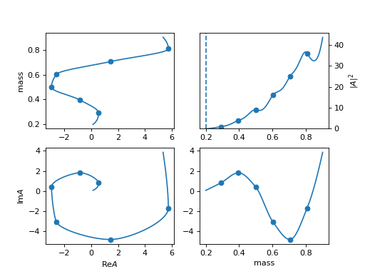
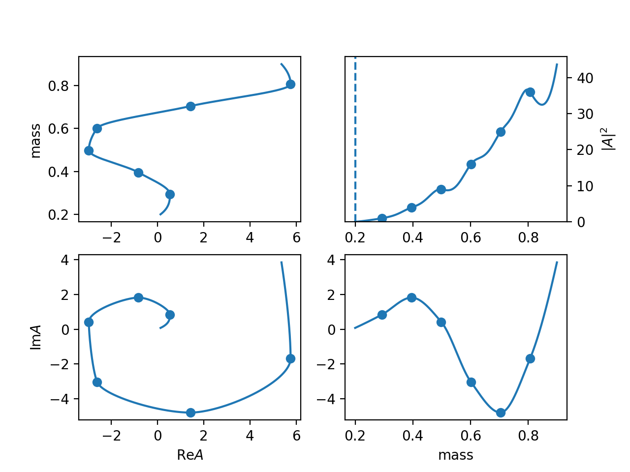
Available Resonances Model
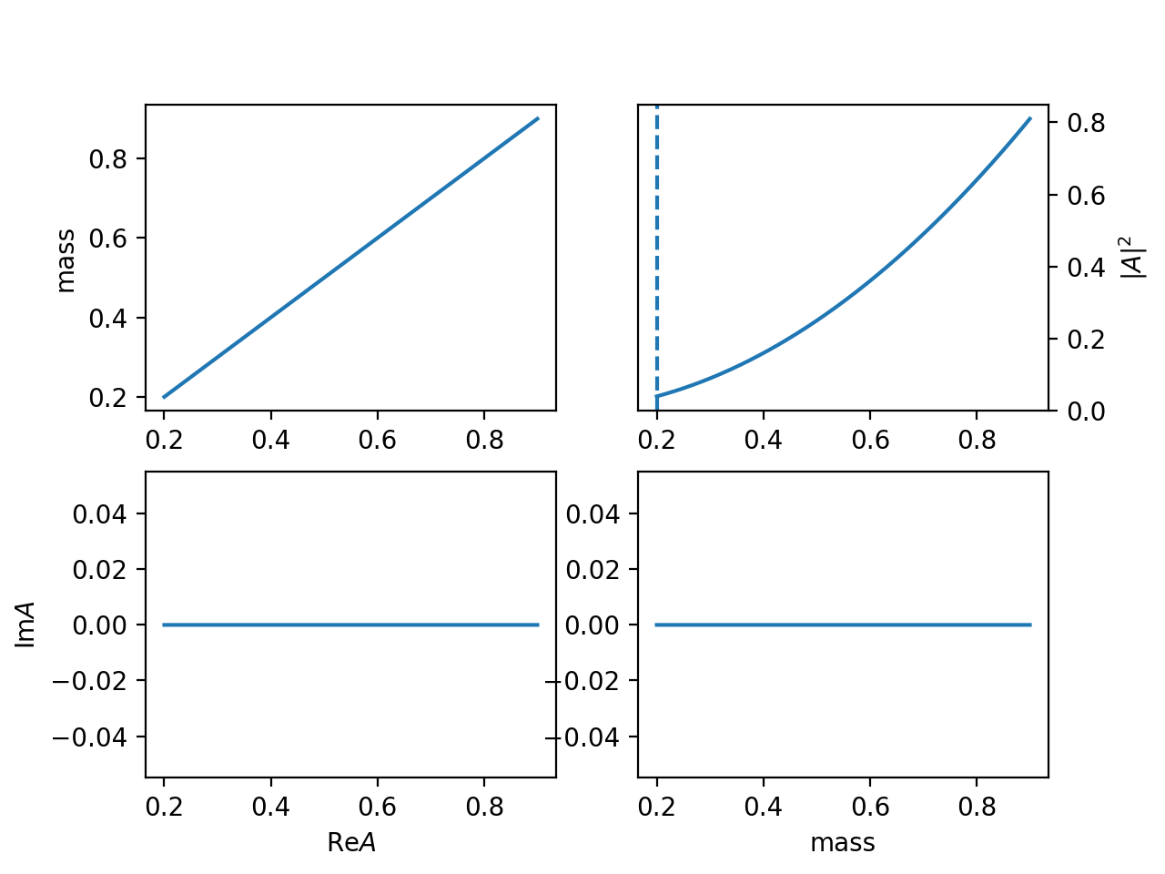
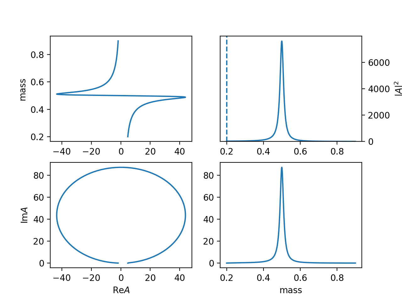
1. "default", "BWR" (Particle)
\[R(m) = \frac{1}{m_0^2 - m^2 - i m_0 \Gamma(m)}\]Argand diagram
(
Source code,png,hires.png,
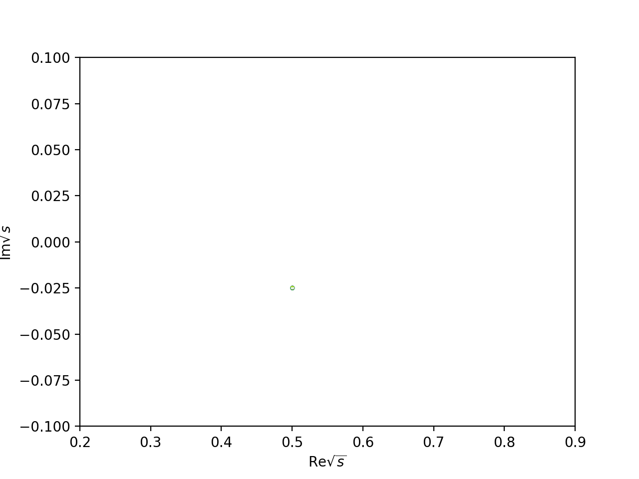
Pole position
(
Source code,png,hires.png,
2. "x" (ParticleX)
simple particle model for mass, (used in expr)
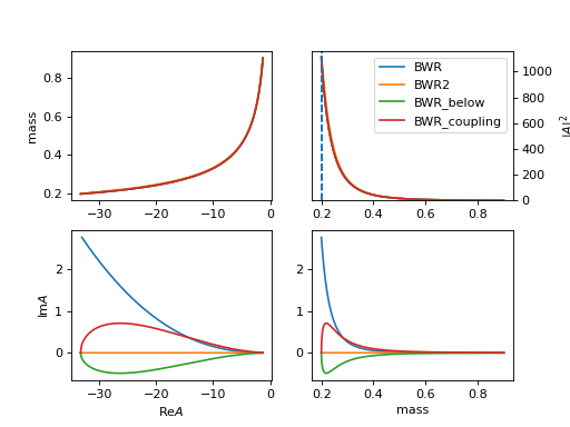
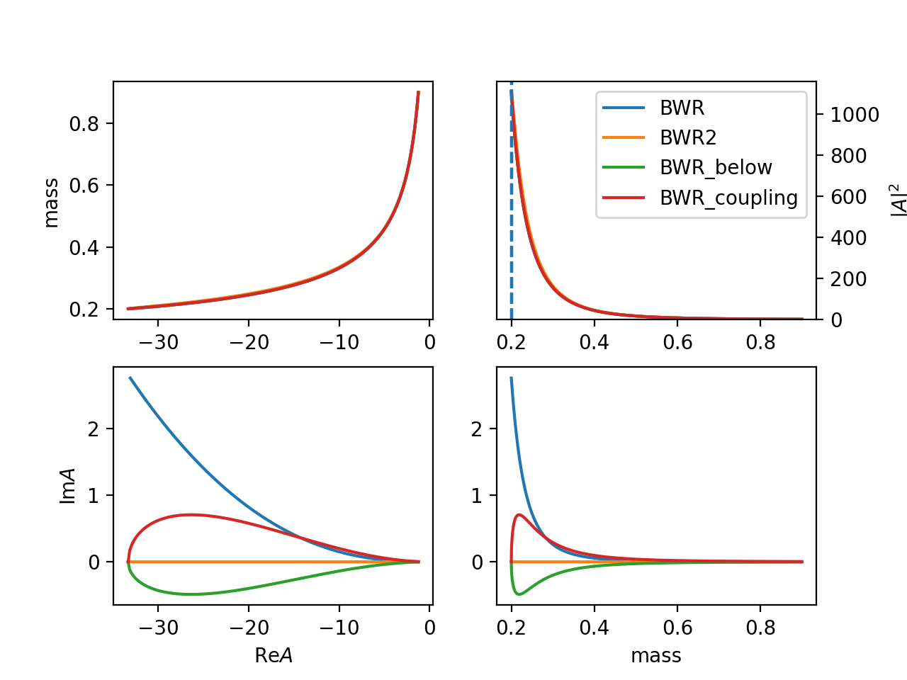
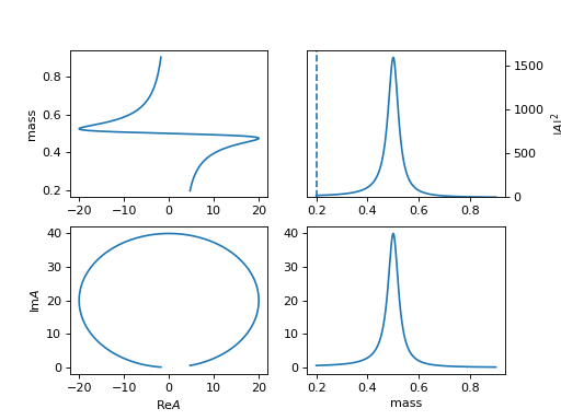
3. "BWR2" (ParticleBWR2)
\[R(m) = \frac{1}{m_0^2 - m^2 - i m_0 \Gamma(m)}\]The difference of
BWR,BWR2is the behavior when mass is below the threshold ( \(m_0 = 0.1 < 0.1 + 0.1 = m_1 + m_2\)).(
Source code,png,hires.png,
4. "BWR_below" (ParticleBWRBelowThreshold)
\[R(m) = \frac{1}{m_0^2 - m^2 - i m_0 \Gamma(m)}\]
5. "BWR_coupling" (ParticleBWRCoupling)
Force \(q_0=1/d\) to avoid below theshold condition for
BWRmodel, and remove other constant parts, then the \(\Gamma_0\) is coupling parameters.\[R(m) = \frac{1}{m_0^2 - m^2 - i m_0 \Gamma_0 \frac{q}{m} q^{2l} B_L'^2(q, 1/d, d)}\](
Source code,png,hires.png,
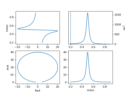
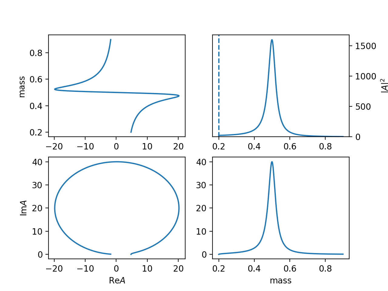
6. "BWR_normal" (ParticleBWR_normal)
\[R(m) = \frac{\sqrt{m_0 \Gamma(m)}}{m_0^2 - m^2 - i m_0 \Gamma(m)}\]
7. "GS_rho" (ParticleGS)
Gounaris G.J., Sakurai J.J., Phys. Rev. Lett., 21 (1968), pp. 244-247
c_daug2Mass: mass for daughter particle 2 (\(\pi^{+}\)) 0.13957039
c_daug3Mass: mass for daughter particle 3 (\(\pi^{0}\)) 0.1349768\[R(m) = \frac{1 + D \Gamma_0 / m_0}{(m_0^2 -m^2) + f(m) - i m_0 \Gamma(m)}\]\[f(m) = \Gamma_0 \frac{m_0 ^2 }{q_0^3} \left[q^2 [h(m)-h(m_0)] + (m_0^2 - m^2) q_0^2 \frac{d h}{d m}|_{m0} \right]\]\[h(m) = \frac{2}{\pi} \frac{q}{m} \ln \left(\frac{m+2q}{2m_{\pi}} \right)\]\[\frac{d h}{d m}|_{m0} = h(m_0) [(8q_0^2)^{-1} - (2m_0^2)^{-1}] + (2\pi m_0^2)^{-1}\]\[D = \frac{f(0)}{\Gamma_0 m_0} = \frac{3}{\pi}\frac{m_\pi^2}{q_0^2} \ln \left(\frac{m_0 + 2q_0}{2 m_\pi }\right) + \frac{m_0}{2\pi q_0} - \frac{m_\pi^2 m_0}{\pi q_0^3}\]
8. "BW" (ParticleBW)

9. "LASS" (ParticleLass)
\[R(m) = \frac{m}{q cot \delta_B - i q} + e^{2i \delta_B}\frac{m_0 \Gamma_0 \frac{m_0}{q_0}} {(m_0^2 - m^2) - i m_0\Gamma_0 \frac{q}{m}\frac{m_0}{q_0}}\]\[cot \delta_B = \frac{1}{a q} + \frac{1}{2} r q\]\[e^{2i\delta_B} = \cos 2 \delta_B + i \sin 2\delta_B = \frac{cot^2\delta_B -1 }{cot^2 \delta_B +1} + i \frac{2 cot \delta_B }{cot^2 \delta_B +1 }\]
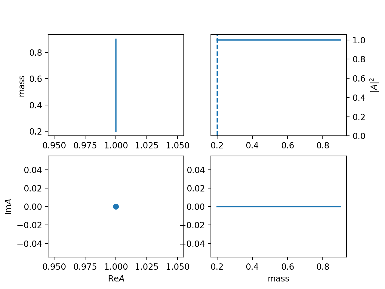
10. "one" (ParticleOne)
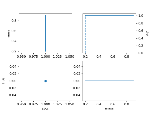
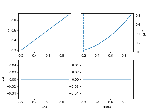
11. "exp" (ParticleExp)
\[R(m) = e^{-|a| m}\]
12. "exp_com" (ParticleExpCom)

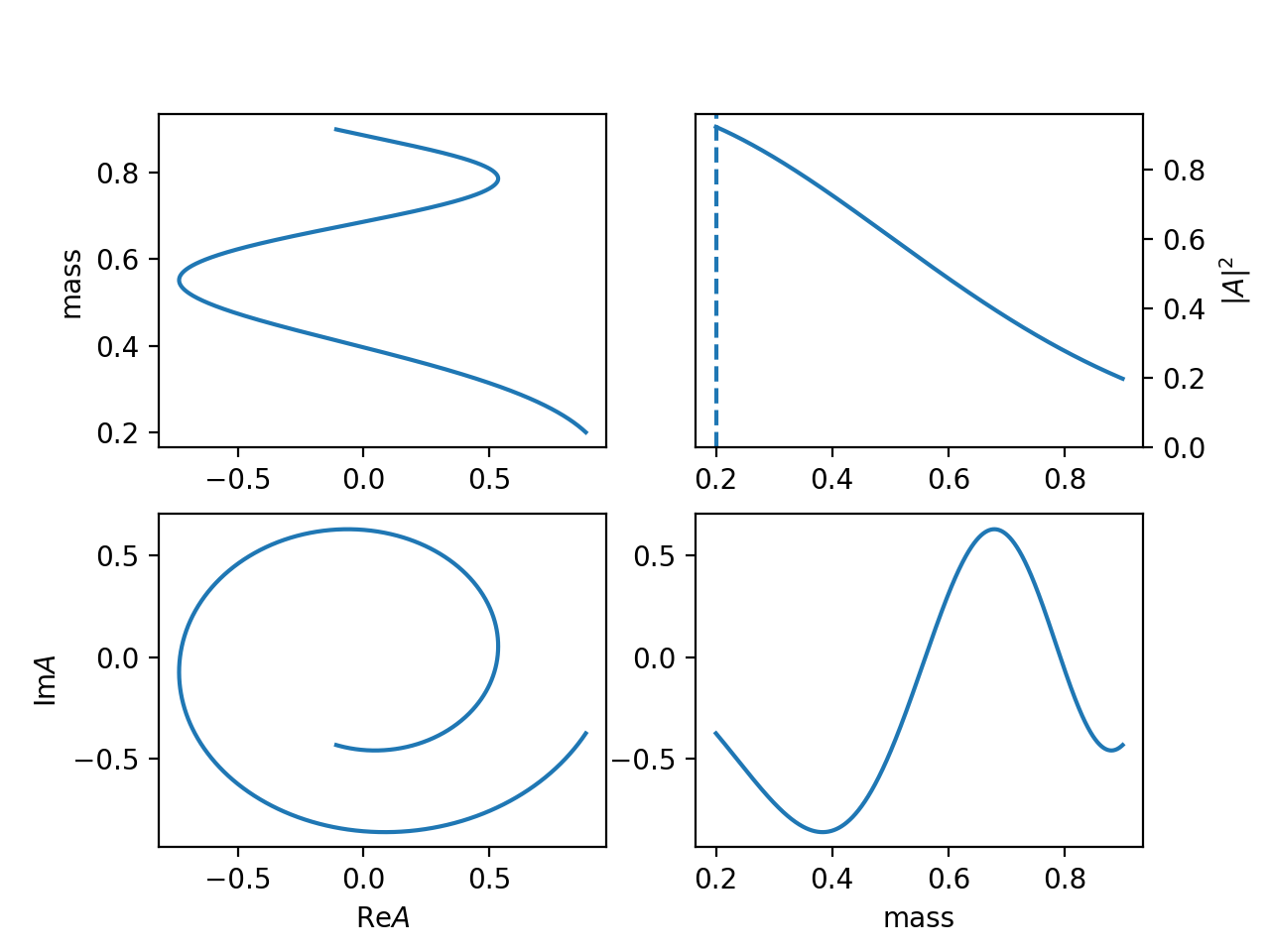
13. "poly" (ParticlePoly)
\[R(m) = \sum c_i (m-m_0)^{n-i}\]lineshape when \(c_0=1, c_1=c_2=0\)
(
Source code,png,hires.png,
14. "MLP" (ParticleMLP)
Multilayer Perceptron like model.
\[R(m) = \sum_{k} w_k activation(m-m_0+b_k)\]lineshape when
interp_N: 11,activation: relu, \(b_k=(k-5)/10\), \(w_k = exp(k i\pi/2)\)(
Source code,png,hires.png,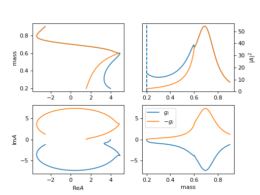
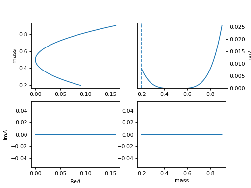
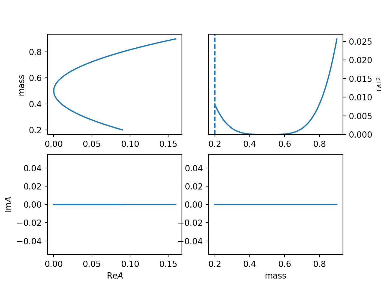
15. "DI" (DispersionIntegralParticle)
Dispersion Integral model. In the model a linear interpolation is used to avoid integration every times in fitting. No paramters are allow in the integration.
\[f(s) = \frac{1}{m_0^2 - s - \sum_{i} g_i^2 [Re\Pi_i(s) -Re\Pi_i(m_0^2) + i Im \Pi_i(s)] }\]where \(Im \Pi_i(s)=\rho_i(s)n_i^2(s)\), \(n_i(s)={q}^{l} {B_l'}(q,1/d, d)\).
The real parts of \(\Pi(s)\) is defined using the dispersion intergral
\[Re \Pi_i(s) = \frac{\color{red}(s-s_{0,i})}{\pi} P \int_{s_{th,i}}^{\infty} \frac{Im \Pi_i(s')}{(s' - s){\color{red} (s'-s_{0,i})}} \mathrm{d} s'\]By default, \(s_{0,i}=0\), it can be change to other value though option
s0: value.value=sthfor \(s_{th,i}\).Note
Small
int_Nwill have bad precision.The shape of \(\Pi(s)\) and comparing to Chew-Mandelstam function \(\Sigma(s)\)
(
Source code,png,hires.png,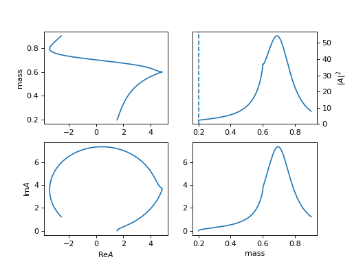
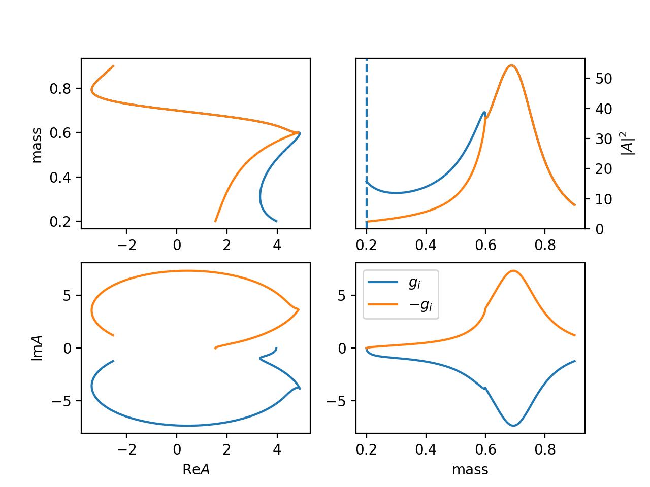
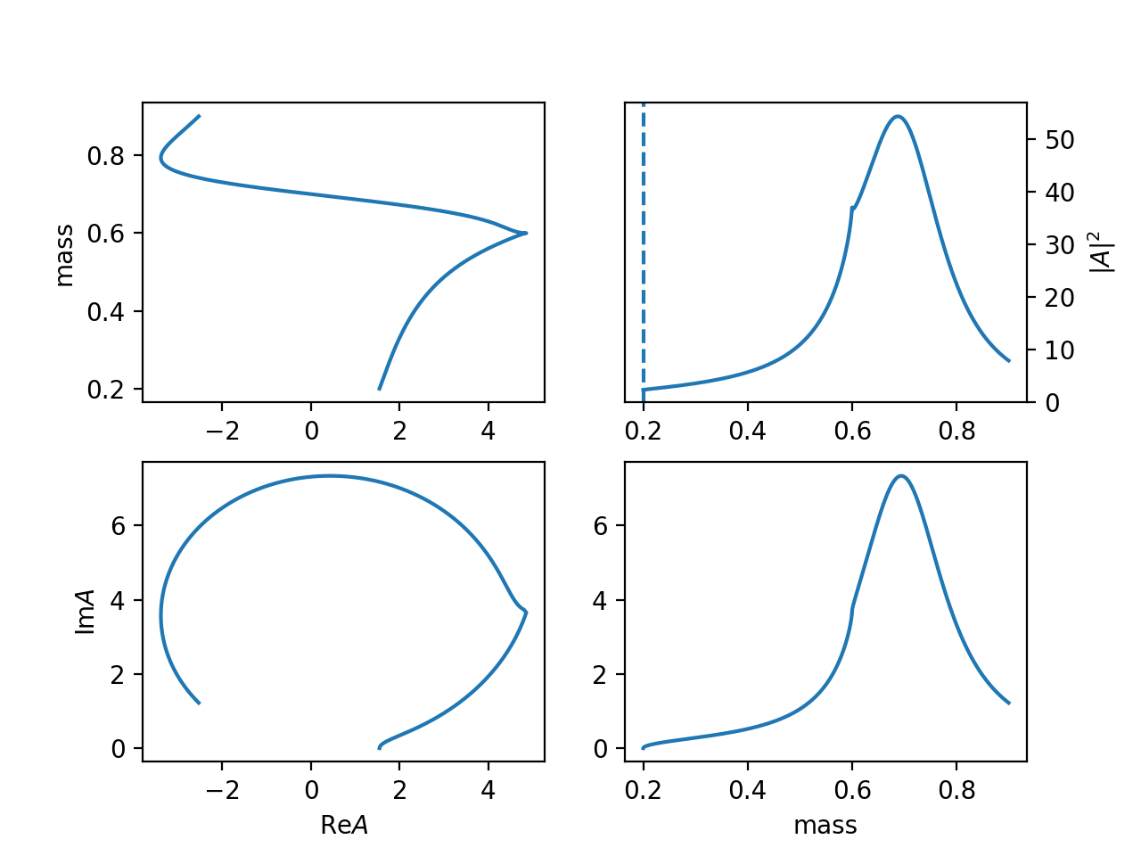
The Argand plot
(
Source code,png,hires.png,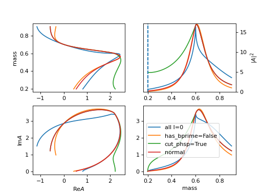
16. "DI_a0" (DispersionIntegralParticleA0)
“DI_a0” model is the model used in PRD78,074023(2008) . In the model a linear interpolation is used to avoid integration every times in fitting. No paramters are allowed in the integration, unless
dyn_int=True.\[f(s) = \frac{1}{m_0^2 - s - \sum_{i} [Re \Pi_i(s) - Re\Pi_i(m_0^2)] - i \sum_{i} \rho'_i(s) }\]where \(\rho'_i(s) = g_i^2 \rho_i(s) F_i^2(s)\) is the phase space with barrier factor \(F_i(s)=\exp(-\alpha k_i^2)\).
The real parts of \(\Pi(s)\) is defined using the dispersion intergral
\[Re \Pi_i(s) = \frac{1}{\pi} P \int_{s_{th,i}}^{\infty} \frac{\rho'_i(s')}{s' - s} \mathrm{d} s' = \lim_{\epsilon \rightarrow 0} \left[ \int_{s_{th,i}}^{s-\epsilon} \frac{\rho'_i(s')}{s' - s} \mathrm{d} s' +\int_{s+\epsilon}^{\infty} \frac{\rho'_i(s')}{s' - s} \mathrm{d} s'\right]\]The reprodution of the Fig1 in PRD78,074023(2008) .
(
Source code,png,hires.png,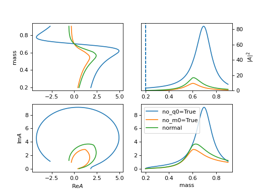
The Argand plot
(
Source code,png,hires.png,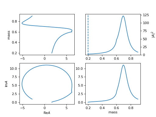
17. "Flatte" (ParticleFlatte)
Flatte like formula
\[R(m) = \frac{1}{m_0^2 - m^2 + i m_0 (\sum_{i} g_i \frac{q_i}{m})}\]\[\begin{split}q_i = \begin{cases} \frac{\sqrt{(m^2-(m_{i,1}+m_{i,2})^2)(m^2-(m_{i,1}-m_{i,2})^2)}}{2m} & (m^2-(m_{i,1}+m_{i,2})^2)(m^2-(m_{i,1}-m_{i,2})^2) >= 0 \\ \frac{i\sqrt{|(m^2-(m_{i,1}+m_{i,2})^2)(m^2-(m_{i,1}-m_{i,2})^2)|}}{2m} & (m^2-(m_{i,1}+m_{i,2})^2)(m^2-(m_{i,1}-m_{i,2})^2) < 0 \\ \end{cases}\end{split}\](
Source code,png,hires.png,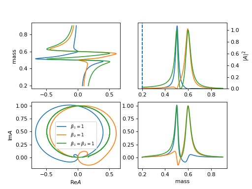
Required input arguments
mass_list: [[m11, m12], [m21, m22]]for \(m_{i,1}, m_{i,2}\).
18. "FlatteC" (ParticleFlatteC)
Flatte like formula
\[R(m) = \frac{1}{m_0^2 - m^2 - i m_0 (\sum_{i} g_i \frac{q_i}{m})}\]\[\begin{split}q_i = \begin{cases} \frac{\sqrt{(m^2-(m_{i,1}+m_{i,2})^2)(m^2-(m_{i,1}-m_{i,2})^2)}}{2m} & (m^2-(m_{i,1}+m_{i,2})^2)(m^2-(m_{i,1}-m_{i,2})^2) >= 0 \\ \frac{i\sqrt{|(m^2-(m_{i,1}+m_{i,2})^2)(m^2-(m_{i,1}-m_{i,2})^2)|}}{2m} & (m^2-(m_{i,1}+m_{i,2})^2)(m^2-(m_{i,1}-m_{i,2})^2) < 0 \\ \end{cases}\end{split}\]Required input arguments
mass_list: [[m11, m12], [m21, m22]]for \(m_{i,1}, m_{i,2}\).(
Source code,png,hires.png,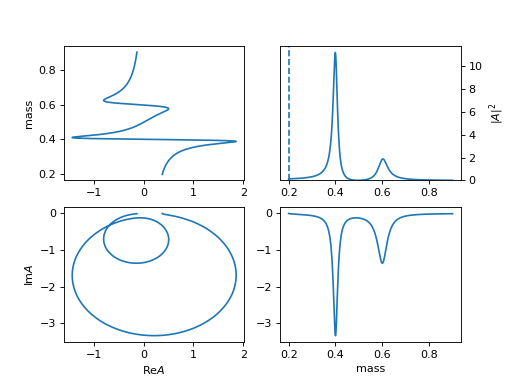
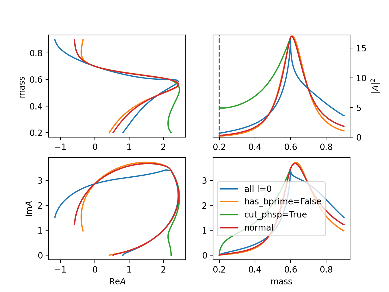
19. "FlatteGen" (ParticleFlateGen)
More General Flatte like formula
\[R(m) = \frac{1}{m_0^2 - m^2 - i m_0 [\sum_{i} g_i \frac{q_i}{m} \times \frac{m_0}{|q_{i0}|} \times \frac{|q_i|^{2l_i}}{|q_{i0}|^{2l_i}} B_{l_i}'^2(|q_i|,|q_{i0}|,d)]}\]\[\begin{split}q_i = \begin{cases} \frac{\sqrt{(m^2-(m_{i,1}+m_{i,2})^2)(m^2-(m_{i,1}-m_{i,2})^2)}}{2m} & (m^2-(m_{i,1}+m_{i,2})^2)(m^2-(m_{i,1}-m_{i,2})^2) >= 0 \\ \frac{i\sqrt{|(m^2-(m_{i,1}+m_{i,2})^2)(m^2-(m_{i,1}-m_{i,2})^2)|}}{2m} & (m^2-(m_{i,1}+m_{i,2})^2)(m^2-(m_{i,1}-m_{i,2})^2) < 0 \\ \end{cases}\end{split}\]Required input arguments
mass_list: [[m11, m12], [m21, m22]]for \(m_{i,1}, m_{i,2}\). And addition argumentsl_list: [l1, l2]for \(l_i\)
has_bprime=Falseto remove \(B_{l_i}'^2(|q_i|,|q_{i0}|,d)\).
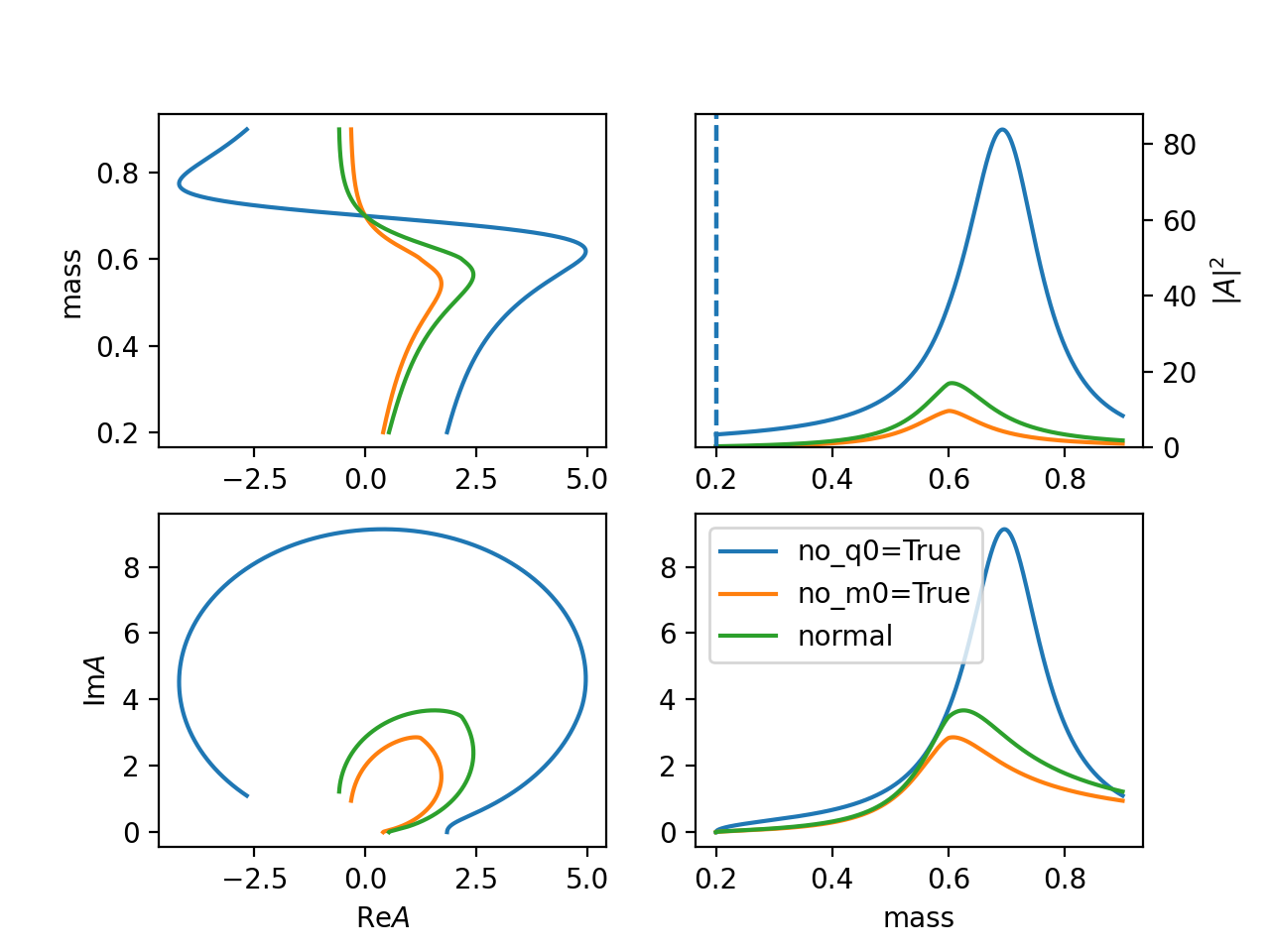
cut_phsp=Trueto set \(q_i = 0\) when \((m^2-(m_{i,1}+m_{i,2})^2)(m^2-(m_{i,1}-m_{i,2})^2) < 0\)The plot use parameters \(m_0=0.7, m_{0,1}=m_{0,2}=0.1, m_{1,1}=m_{1,2}=0.3, g_0=0.3,g_1=0.2,l_0=0,l_1=1\).
(
Source code,png,hires.png,
no_m0=Trueto set \(i m_0 => i\) in the width part.
no_q0=Trueto remove \(\frac{m_0}{|q_{i0}|}\) and set others \(q_{i0}=1\).(
Source code,png,hires.png,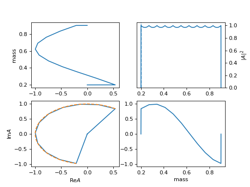
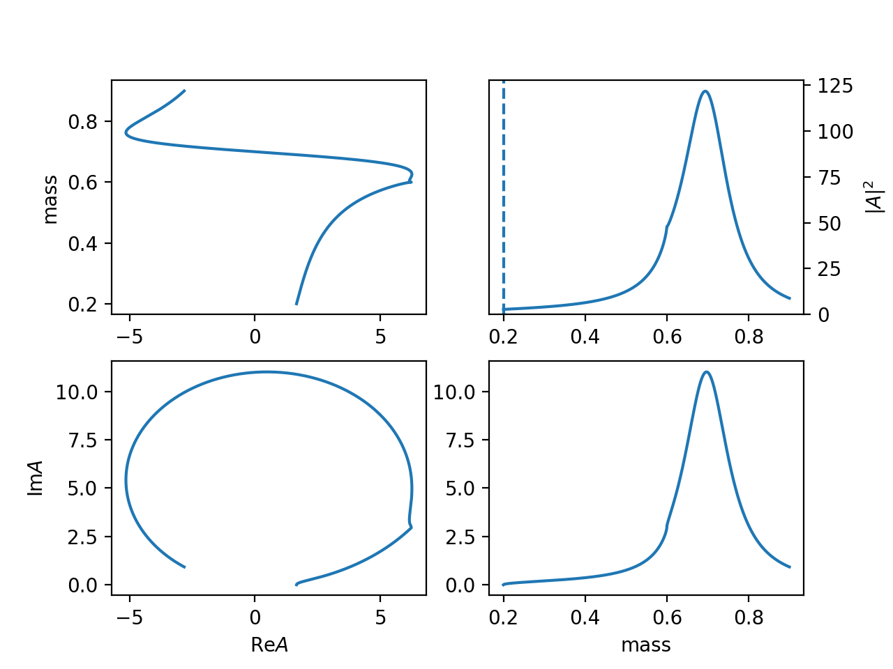
20. "Flatte2" (ParticleFlate2)
General Flatte like formula.
\[R(m) = \frac{1}{m_0^2 - m^2 - i m_0 [\sum_{i} \color{red}{g_i^2}\color{black} \frac{q_i}{m} \times \frac{m_0}{|q_{i0}|} \times \frac{|q_i|^{2l_i}}{|q_{i0}|^{2l_i}} B_{l_i}'^2(|q_i|,|q_{i0}|,d)]}\]\[\begin{split}q_i = \begin{cases} \frac{\sqrt{(m^2-(m_{i,1}+m_{i,2})^2)(m^2-(m_{i,1}-m_{i,2})^2)}}{2m} & (m^2-(m_{i,1}+m_{i,2})^2)(m^2-(m_{i,1}-m_{i,2})^2) >= 0 \\ \frac{i\sqrt{|(m^2-(m_{i,1}+m_{i,2})^2)(m^2-(m_{i,1}-m_{i,2})^2)|}}{2m} & (m^2-(m_{i,1}+m_{i,2})^2)(m^2-(m_{i,1}-m_{i,2})^2) < 0 \\ \end{cases}\end{split}\]It has the same options as
FlatteGen.(
Source code,png,hires.png,
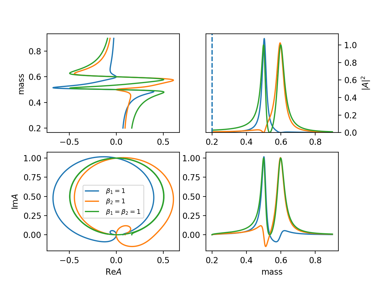
21. "KMatrixSingleChannel" (KmatrixSingleChannelParticle)
K matrix model for single channel multi pole.
\[K = \sum_{i} \frac{m_i \Gamma_i(m)}{m_i^2 - m^2 }\]\[P = \sum_{i} \frac{\beta_i m_0 \Gamma_0 }{ m_i^2 - m^2}\]the barrier factor is included in gls
\[R(m) = (1-iK)^{-1} P\]requird
mass_list: [pole1, pole2]andwidth_list: [width1, width2].(
Source code,png,hires.png,
22. "KMatrixSplitLS" (KmatrixSplitLSParticle)
K matrix model for single channel multi pole and the same channel with different (l, s) coupling.
\[K_{a,b} = \sum_{i} \frac{m_i \sqrt{\Gamma_{a,i}(m)\Gamma_{b,i}(m)}}{m_i^2 - m^2 }\]\[P_{b} = \sum_{i} \frac{\beta_i m_0 \Gamma_{b,i0} }{ m_i^2 - m^2}\]the barrier factor is included in gls
\[R(m) = (1-iK)^{-1} P\]
23. "KmatrixSimple" (KmatrixSimple)
simple Kmatrix formula.
K-matrix
\[K_{i,j} = \sum_{a} \frac{g_{i,a} g_{j,a}}{m_a^2 - m^2+i\epsilon}\]P-vector
\[P_{i} = \sum_{a} \frac{\beta_{a} g_{i,a}}{m_a^2 - m^2 +i\epsilon} + f_{bkg,i}\]total amplitude
\[R(m) = n (1 - K i \rho n^2)^{-1} P\]barrief factor
\[n_{ii} = q_i^l B'_l(q_i, 1/d, d)\]phase space factor
\[\rho_{ii} = q_i/m\]\(q_i\) is 0 when below threshold
24. "BWR_LS" (ParticleBWRLS)
Breit Wigner with split ls running width
\[R_i (m) = \frac{g_i}{m_0^2 - m^2 - im_0 \Gamma_0 \frac{\rho}{\rho_0} (\sum_{i} g_i^2)}\], \(\rho = 2q/m\), the partial width factor is
\[g_i = \gamma_i \frac{q^l}{q_0^l} B_{l_i}'(q,q_0,d)\]and keep normalize as
\[\sum_{i} \gamma_i^2 = 1.\]The normalize is done by (\(\cos \theta_0, \sin\theta_0 \cos \theta_1, \cdots, \prod_i \sin\theta_i\))
25. "BWR_LS2" (ParticleBWRLS2)
Breit Wigner with split ls running width, each one use their own l,
\[R_i (m) = \frac{1}{m_0^2 - m^2 - im_0 \Gamma_0 \frac{\rho}{\rho_0} (g_i^2)}\], \(\rho = 2q/m\), the partial width factor is
\[g_i = \gamma_i \frac{q^l}{q_0^l} B_{l_i}'(q,q_0,d)\]
26. "MultiBWR" (ParticleMultiBWR)

27. "MultiBW" (ParticleMultiBW)
Combine Multi BW into one particle
28. "linear_npy", "linear_txt" (InterpLinearNpy)
Linear interpolation model from a
txtfile with array of [mi, re(ai), im(ai)]. Requiredfile: path_of_file.txt, for the path oftxtfile. It also supportnpyfile.The example is
exp(5 I m).(
Source code,png,hires.png,
29. "width_linear_npy", "width_linear_txt" (WidthInterpLinearNpy)
Linear interpolation model from a
txtfile with array of [mi, re(gi), im(gi)]. Requiredfile: path_of_file.txt, for the path oftxtfile. It also supportnpyfile.Using interpolation for \(\Pi(m)\).
\[f(m) = \frac{1}{m_0^2 - m^2 - m_0 \Gamma_0 (Re \Pi(m) - Re \Pi(m_0) + i Im \Pi(m))}\]Additional option
width_scale: True, will use \(\Pi(m)/Im \Pi(m_0)\) instead of \(\Pi(m)\) to have a normal width value.The example is
exp(5 I m).(
Source code,png,hires.png,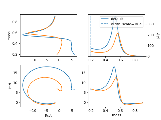
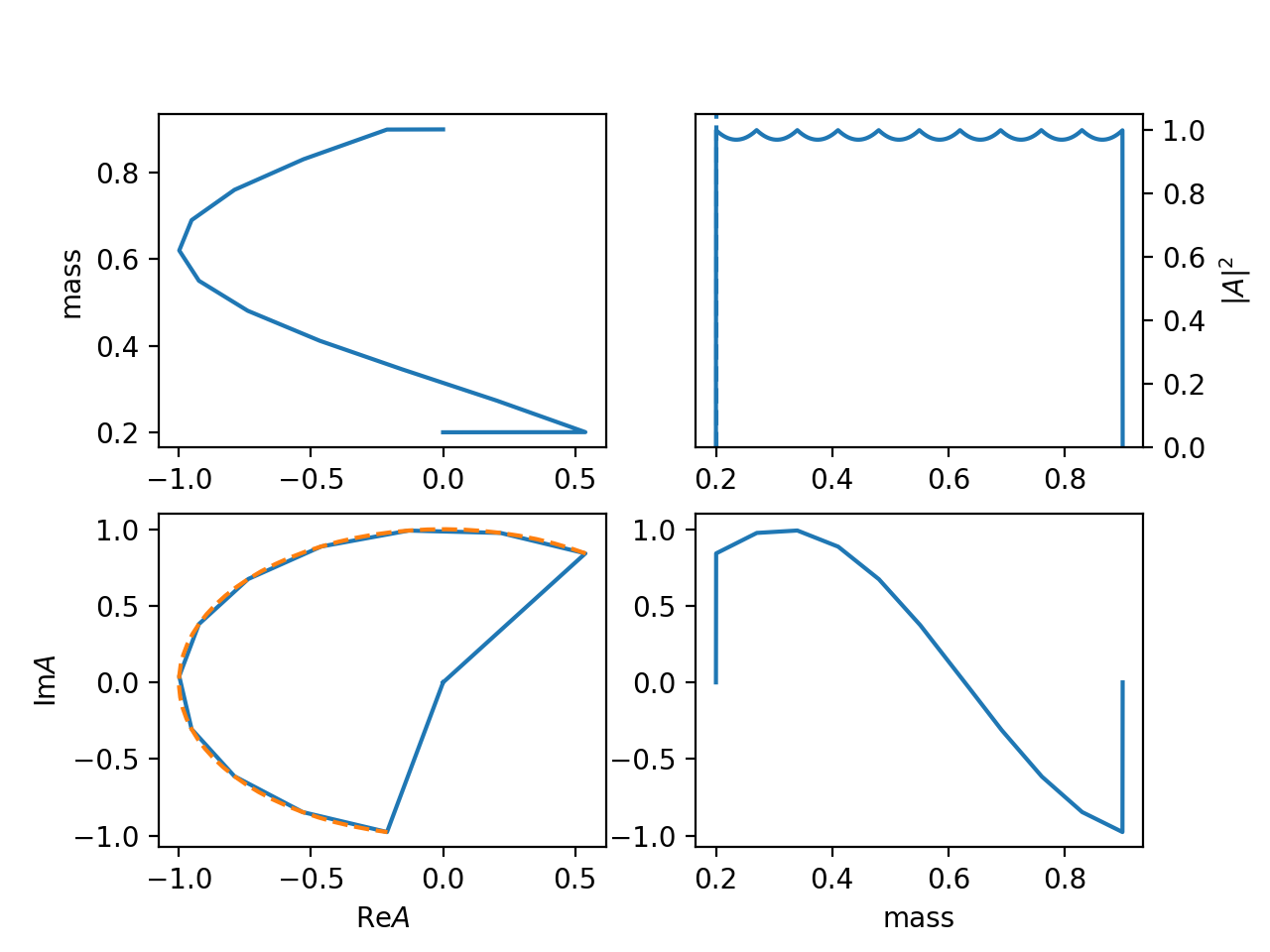
30. "interp" (Interp)
linear interpolation for real number
31. "interp_c" (Interp)
linear interpolation for complex number
32. "spline_c" (Interp1DSpline)
Spline interpolation function for model independent resonance
33. "interp1d3" (Interp1D3)
Piecewise third order interpolation
34. "interp_lagrange" (Interp1DLang)
Lagrange interpolation
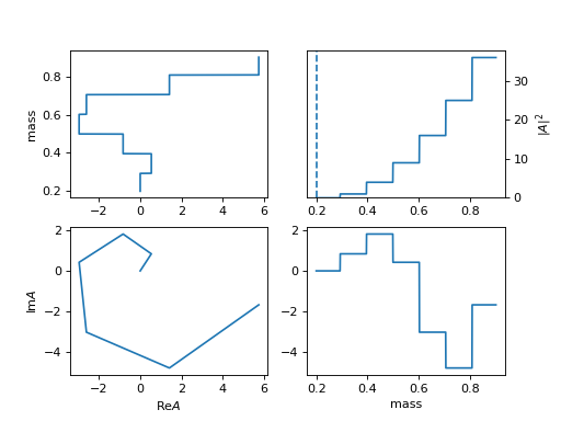
35. "interp_hist" (InterpHist)
Interpolation for each bins as constant
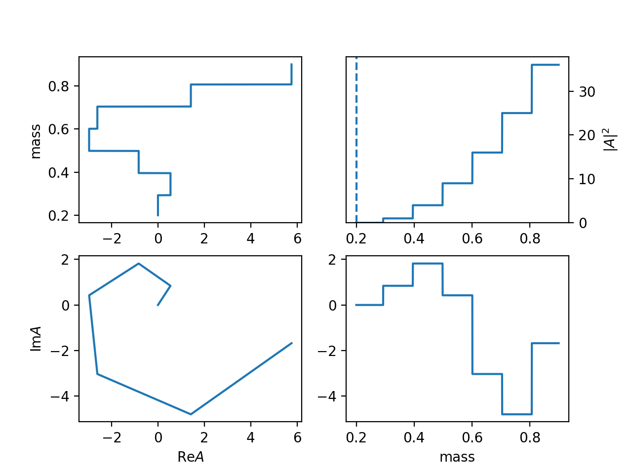
36. "hist_idx" (InterpHistIdx)
Interpolation for each bins as constant
use
min_m: 0.19
max_m: 0.91
interp_N: 8
with_bound: True
for mass range [0.19, 0.91] and 7 bins
The first and last are fixed to zero unless set
with_bound: True.This is an example of \(k\exp (i k)\) for point k.
(
Source code,png,hires.png,
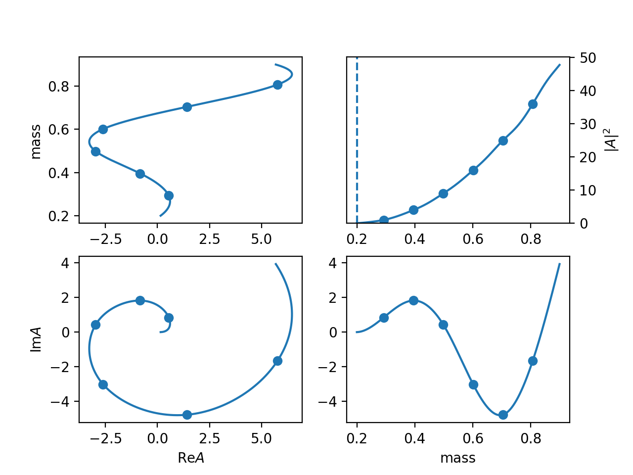
37. "spline_c_idx" (Interp1DSplineIdx)
Spline function in index way.
use
min_m: 0.19
max_m: 0.91
interp_N: 8
with_bound: True
for mass range [0.19, 0.91] and 8 interpolation points
The first and last are fixed to zero unless set
with_bound: True.This is an example of \(k\exp (i k)\) for point k.
(
Source code,png,hires.png,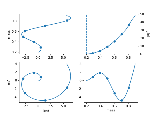
38. "sppchip" (InterpSPPCHIP)
Shape-Preserving Piecewise Cubic Hermite Interpolation Polynomial. It is monotonic in each interval.
(
Source code,png,hires.png,